Data-efficient HHMM

This notebook contains code to simulate data from a data-efficient hierarchical hidden Markov model (HHMM) and then fit a model to the simulated data.

1. Create a model

We’ll start by creating a random model with 5 high-level states and 20 syllables. The model parameters consist of three matrices:

• trans_probs: transition probabilities between hidden states

• emission_base: baseline transition matrix for syllables (in a low-rank format)

• emission_biases: syllable transition biases imposed by the hidden states (in a low-rank format)

from state_moseq.hhmm_efficient import random_params
import matplotlib.pyplot as plt
import jax.random as jr
import jax.numpy as jnp
import numpy as np

hypparams = {
    "n_states": 5,
    "emission_base_sigma": 1,
    "emission_biases_sigma": 1,
    "trans_beta": 1,
    "trans_kappa": 100,
    "n_syllables": 20,
    "emission_gd_iters": 500,
    "emission_gd_lr": 1e-2,
}
simulation_params = random_params(jr.PRNGKey(0), hypparams)

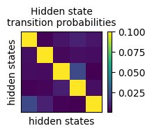
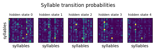
2. Visualize model parameters

The code below plots trans_probs as well as full-rank syllable transition matrices that come from combining emission_base and emission_biases.

plt.imshow(simulation_params["trans_probs"], vmax=0.1)
plt.colorbar()
plt.xlabel("hidden states")
plt.ylabel("hidden states")
plt.title('Hidden state\ntransition probabilities', fontsize=10)
plt.xticks([])
plt.yticks([])
plt.gcf().set_size_inches((2,1.5))

from state_moseq.hhmm_efficient import get_syllable_trans_probs

syllable_trans_probs = get_syllable_trans_probs(
    simulation_params["emission_base"],
    simulation_params["emission_biases"]
)
fig,axs = plt.subplots(1, hypparams["n_states"], sharey=True)
for i in range(hypparams["n_states"]):
    axs[i].imshow(syllable_trans_probs[i])
    axs[i].set_xlabel("syllables")
    axs[i].set_xticks([])
    axs[i].set_title(f'hidden state {i}', fontsize=8)
axs[0].set_yticks([])
axs[0].set_ylabel("syllables")
fig.subplots_adjust(top=1.45)
fig.suptitle("Syllable transition probabilities");

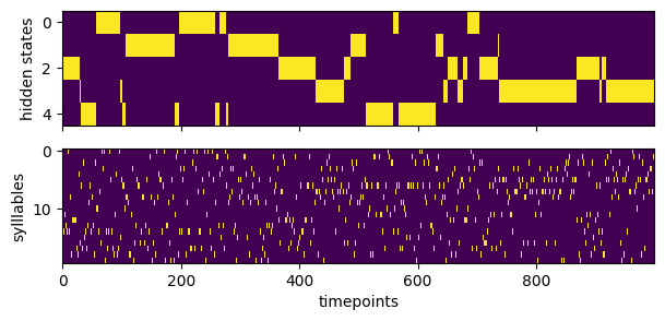
3. Simulate data from model

Now let’s generate fake data from the model. The simulation will first sample a sequence higher order states and then use those to generate a sequence of syllables.

from state_moseq.hhmm_efficient import simulate

n_sequences = 200
n_timesteps = 1000

true_states, syllables = simulate(
    jr.PRNGKey(2), simulation_params, n_timesteps, n_sequences
)

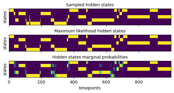
Visualize example “recording”

fig,axs = plt.subplots(2,1,sharex=True)
axs[0].imshow(np.eye(hypparams["n_states"])[true_states[0]].T, aspect='auto', interpolation='none')
axs[0].set_ylabel("hidden states")
axs[1].imshow(np.eye(hypparams["n_syllables"])[syllables[0]].T, aspect='auto', interpolation='none')
axs[1].set_ylabel("sylllables")
axs[1].set_xlabel("timepoints")
fig.set_size_inches((7,3))

4. Perform inference

Next we’ll try to infer the model parameters from the simulated data using Gibbs sampling. Before inference, we have to generate a data dictionary that contains syllables and an array called mask. The purpose of mask is to indicate missing data in the syllables array and is useful when modeling sequences of uneven length. In our case there is no missing data so mask will be all 1’s.

from state_moseq.hhmm_efficient import initialize_params, fit_gibbs

data = {
    "syllables": syllables,
    "mask": jnp.ones_like(syllables),
}

# initial guess for parameters
init_params = initialize_params(data, hypparams, seed=jr.PRNGKey(3))

params, states, log_joints = fit_gibbs(
    data,
    hypparams,
    init_params,
    num_iters = 100)

100%|█████████████████████████████████████████| 100/100 [00:09<00:00, 10.55it/s]

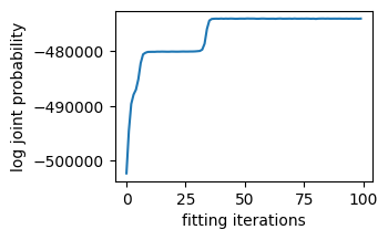
Check for convergence

To make sure the model converged, we’ll check for a plateau in the log joint probability

plt.plot(log_joints)
plt.ylabel('log joint probability')
plt.xlabel('fitting iterations')
plt.gcf().set_size_inches((3,2))

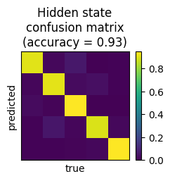
5. Inspect model fit

To compare true vs. inferred hidden states, the following code:

• Generates and plots a confusion matrix

• Calculates the accuracy, defined as the proportion of correctly classified timepoints (after permutation)

from state_moseq import compare_states

confusion, permutation, accuracy = compare_states(states, true_states, hypparams["n_states"])

plt.imshow(confusion[permutation], vmin=0)
plt.colorbar()
plt.title(f'Hidden state\nconfusion matrix\n(accuracy = {round(accuracy.item(),2)})')
plt.xticks([])
plt.yticks([])
plt.ylabel("predicted")
plt.xlabel("true")
plt.gcf().set_size_inches((2.5,2))

6. Hidden state estimation

The states variable returned by fit_gibbs is the output of the final Gibbs sampling step. At best, this represents a random sample from the model’s posterior distribution. In some cases, it may also be useful to estimate the maximum likelihood sequence of hidden states and/or the marginal distribution of hidden states at each timepoint.

from state_moseq.hhmm_efficient import predicted_states, smoothed_states

maximum_likelihood_states = predicted_states(data, params)
marginal_probabilities = smoothed_states(data, params)

fig,axs = plt.subplots(3,1,sharex=True)
axs[0].imshow(np.eye(hypparams["n_states"])[states[0]].T, aspect='auto', interpolation='none')
axs[0].set_title("Sampled hidden states", fontsize=10)
axs[1].imshow(np.eye(hypparams["n_states"])[maximum_likelihood_states[0]].T, aspect='auto', interpolation='none')
axs[1].set_title("Maximum likelihood hidden states", fontsize=10)
axs[2].imshow(marginal_probabilities[0].T, aspect='auto', interpolation='none')
axs[2].set_title("Hidden states marginal probabilities", fontsize=10)
axs[2].set_xlabel("timepoints")
for ax in axs:
    ax.set_ylabel("states")
    ax.set_yticks([])
fig.subplots_adjust(hspace=.6)
fig.set_size_inches((7,3))

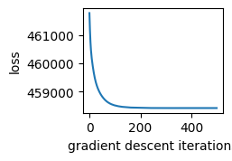
7. Check gradient descent

The syllable emission parameters are estimated using gradient descent. One useful step for debugging is to check for convergence of this step.

from state_moseq.hhmm_efficient import resample_params

_, gd_losses = resample_params(jr.PRNGKey(0), data, params, states, hypparams)

plt.plot(gd_losses)
plt.xlabel('gradient descent iterations')
plt.ylabel('loss')
plt.gcf().set_size_inches((2,1.5))